𝐋𝐋𝐌𝐬 𝐀𝐫𝐞 𝐈𝐦𝐩𝐫𝐞𝐬𝐬𝐢𝐯𝐞. 𝐁𝐮𝐭 𝐀𝐫𝐞 𝐒𝐋𝐌𝐬 𝐌𝐨𝐫𝐞 𝐏𝐫𝐚𝐜𝐭𝐢𝐜𝐚𝐥 𝐟𝐨𝐫 𝐁𝐮𝐬𝐢𝐧𝐞𝐬𝐬?
Study of Modal Characteristics of a System using K-nearest neighbors: Machine Learning Approach
Introduction
The study of modal characteristics is important to determine the natural frequencies of the system. In this study, a four DOF (degrees-of-freedom) system as shown in figure 1 is studied for the parameters tabulated in table 1. The mass, stiffness and damping matrices for the whole system are calculated and finally, the frequency response function is calculated to observe the resonant frequencies of the system.
A data set is prepared by modifying the mass and the parallel stiffness of the system for a different set of values and the respective first resonant frequencies are recorded. Latin hypercube sampling is used to optimally distribute the data points (mass & stiffness) in the design space, to prepare the data.
The data obtained is trained using KNN (k-nearest neighbors regression) by selecting an optimal value of k. The trained KNN is used to predict the resonant frequency of a new set of mass and stiffness. It was observed that the prediction is close to the actual value.
Modal Analysis
The dynamic equation of motion, global mass, stiffness and damping matrices for the 4 DOF system are derived in the following way.
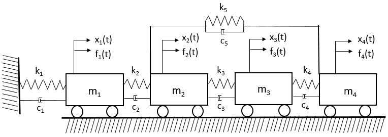 |
| Figure 1: 4 DOF System |
|
DOF number |
Mass (kg) |
Stiffness (N/m) |
|
1 |
125 |
10e6 |
|
2 |
75 |
10.2e6 |
|
3 |
45 |
21e6 |
|
4 |
15 |
9.5e6 |
|
5 |
|
5e4 |
Proportion coefficient to mass matrix, a = 0.5
Proportion coefficient to stiffness matrix, b = 0.00001
The equations of motion for each mass are derived in the following way.

Writing the mass, stiffness and damping matrices according to the following relation.

The frequency response function, Accelerance is generated for a frequency range of 1-200 Hz by converting the dynamic equation of motion into laplace domain. The generated accelerance plots for various inputs and outputs shows the resonant frequencies of the system as depicted in figure 2, 3 & 4.
 |
| Figure 2 :Accelerance - Input at DOF4, Output at DO4 |
 |
| Figure 3: Accelerance - Input at DOF2, Output at DO2 |
 |
| Figure 4: Accelerance - Input at DOF2, Output at DO4 |
Machine Learning
 |
| Figure 5: DOE LHS |
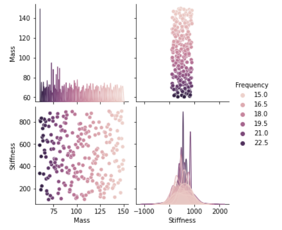 |
| Figure 6: Statistical distribution of variables |
The data prepared from the design of experiments (DOE) is trained using the KNN regression technique by splitting into 80% as a training set and 20% as a testing test, randomly selecting the samples from the data.
Initially, the number of nearest neighbors, i.e., k, is randomly selected and the algorithm is implemented by calculating the euclidean distances between the test set and the training set. The prediction was acceptable but not great and hence a study is carried out to find out the optimal value of k. The training is performed for the k values ranging from 1 to 40 and the error in each case is plotted as shown in figure 7.
 |
| Figure 7: k neighbors Vs prediction error |
From figure 7, it was observed that the error is initially increased and locally minimized when the value of k is equal to 2. The error kept increasing with the value of k and there is a minima again when the value of k is equal to 9 and 10 and further increased with k.
The prediction is performed on the test set with the k values of 2 and 10. It was observed that the 2 nearest neighbors are under-predicting the result and hence 10 nearest neighbors are chosen. Three experiments are carried out on a new set of mass and stiffness to predict the first natural frequency and the results are compared with the actual values. It was observed that the algorithm has well predicted the result which can be seen in figure 8.
 |
| Figure 8: Prediction Vs Actual |
Subscribe to:
Posts (Atom)
-
 Objective and Overview This study aims at predicting the maximum pressure in a hydrodynamic plane slider pad bearing using Machine Learni...
 -
𝐋𝐋𝐌𝐬 𝐀𝐫𝐞 𝐈𝐦𝐩𝐫𝐞𝐬𝐬𝐢𝐯𝐞. 𝐁𝐮𝐭 𝐀𝐫𝐞 𝐒𝐋𝐌𝐬 𝐌𝐨𝐫𝐞 𝐏𝐫𝐚𝐜𝐭𝐢𝐜𝐚𝐥 𝐟𝐨𝐫 𝐁𝐮𝐬𝐢𝐧𝐞𝐬𝐬? In the past few weeks, I...
-
Objective This study aims at determining the pressure distribution in a hydrodynamic plane slider pad bearing. A study of bearings and it...

"Are Large Language Models (LLMs) truly the future of enterprise transformation, or can Small Language Models (SLMs) meet most needs more effectively for specific, tailored use cases?"
Here is my analysis so far (still a work in progress):
LLMs like GPT-4 and Claude 3.5 Sonnet contain 175 billion to over 1 trillion parameters requiring massive distributed computing infrastructure. Small language models, typically 1-20 billion parameters like Llama 3.2, Gemini Nano, sacrifice some general knowledge breadth for dramatic gains in efficiency, speed and cost-effectiveness.
Here's the interesting part:
For many enterprise scenarios, smaller models aren't a compromise—they're a strategic advantage. A fine-tuned 7B parameter model focused on a specific domain can outperform GPT-4 on specialized tasks, all while costing 10x to 50x less to operate.
(Source: https://lnkd.in/erjTAnWu)
Premium LLM APIs can cost $75 per million input tokens for GPT 4.5, while SLMs like Llama can operate at around $0.03 for the same.
Adding to this, LLMs often require GPU clusters worth hundreds of thousands of dollars, whereas SLMs can run efficiently on local machines under $10,000.
Most importantly, latency often matters more than the capability.
SLMs deliver 6-10 tokens per second on modest hardware making them ideal for real-time applications. LLMs, despite their power, typically require 5-30 seconds for complex responses and introduce variable latency due to distributed processing. For applications where users expect immediate feedback, this performance gap becomes a competitive disadvantage regardless of the model's theoretical capabilities.
So unless, there is a strong need for strategic analysis or multi-step reasoning, is there a real need for LLMs in enterprise applications?
Follow the blog for detailed analysis in the next post.