Objective
This study aims at determining the
pressure distribution in a hydrodynamic plane slider pad bearing. A study of
bearings and its types can be found in this article.
Method
Numerical methods are widely used to
solve differential equations and find an approximate solution. Finite
difference method (FDM) is one of the numerical methods where the differential
operators are converted into algebraic equations at the grid points of the
computational domain and are solved for the values using the gauss elimination
or the matrix inversion method.
The differential equations are
converted into algebraic equations in the following way.

Where i represents the node number in
the grid in x direction (since y varies with respect x).

In the above equations, y is varying only with
respect to x. If it is varying with some variable, say 'z', then the
problem turns out to be a two-dimensional case where finite difference
equations have to be applied along the 'z' direction as well.
Problem definition and Solution
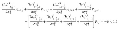
Reynold’s equation is used to determine the pressure distribution. The governing differential equations is considered as follows.

Here, the pressure variation is to be
determined along ‘x’ (length of the bearing) and ‘y’ (width of
the bearing) directions. The height of the bearing is driven by the function ‘h’.
Newtonian fluid is considered in
laminar flow and assumed to be incompressible, hence the density remains
constant. Also, temperature variation is neglected so the viscosity also
remains constant.
From the computational point of view,
it is advisable to non-dimensionalize the entities and solve the problem. Hence
the equivalent non-dimensional form of the Reynold’s equation is as follows.

The above equation is transformed into
a Finite difference equation in two-dimensional form where ‘i’
represents the grid in x0 direction and ‘j’ represents
the grid in y0 direction.
The height of the bearing is given by
2.5-1.5*x0 which is a function of x0. Grid
is spaced from 0 to 1 in x0 direction and 0 to 0.5 in y0 direction.
The computational domain is divided into equally spaced 30 nodes in x0 and y0 directions. The element size is determined after achieving the convergence of the mesh or grid. The grid can be seen in the figure below.
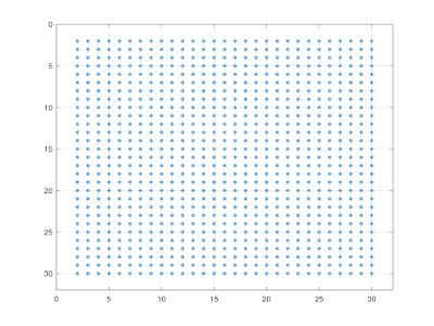 |
| Computational domain |
Dirichlet boundary condition is applied where the pressure is zero at the boundaries of the computational domain. The height functions are calculated at every node of the grid as per the finite difference equations and finally the pressure of the computational domain is determined which can be seen in the figure below.
 |
| Non-dimensional pressure distribution |
The maximum value of the non-dimensional pressure is 0.0016034 converted to dimensional pressure, the value is 5.3 KPa. The dimensional pressure distribution can be seen in the figure below.
 |
| Dimensional pressure distribution |

